EXPLAIN (ANALYZE) needs BUFFERS to improve the Postgres query optimization process

Jupiter's moon IO. Credit: ALMA (ESO/NAOJ/NRAO), I. de Pater et al.; NRAO/AUI NSF, S. Dagnello; NASA/JPL/Space Science Institute
SQL query optimization is challenging for those who have just started working with PostgreSQL. There are many objective reasons for this, such as:
- the difficulty of the field of system performance in general,
- lack of good "playground" environments where people can experience how databases work at a larger scale,
- lack of certain capabilities in Postgres observability tools that are still developing (though, at a good pace),
- insufficiency of good educational materials.
All these barriers are reasonable. They limit the number of engineers possessing well-developed Postgres query optimization skills. However, there is a specific artificial barrier that is rather influential and which is relatively easy to eliminate.
Here it is: the EXPLAIN command has the BUFFERS option disabled by default. I am sure it has to be enabled and used by everyone who needs to do some SQL optimization work.
EXPLAIN ANALYZE or EXPLAIN (ANALYZE, BUFFERS)?
The BUFFERS option helps us see how much IO work Postgres did when executing each node in the query execution plan. For database systems, which mostly perform IO-intensive operations, dealing with too many data pages (or "buffers", "blocks" – depending on the context) is the most popular reason for poor performance.
Further, we will consider several examples of EXPLAIN (ANALYZE) plans and discuss why everyone needs to use the BUFFERS option when troubleshooting the performance of a particular query.
1) Seeing the IO work done
Let's consider a simple example – two tables, each has 2 bigint columns, id (sequential) and num (random), with exactly the same content; the second table has an index on num while the first one doesn't have it:
create table t1 as
select id::int8, round(random() * 100000)::int8 as num
from generate_series(1, 10000000) as id;

create table t2 as select * from t1;

alter table t1 add primary key (id);
alter table t2 add primary key (id);

create index i_t2_num on t2 using btree (num);

vacuum analyze t1;
vacuum analyze t2;
Result:
test=# \d t1
                  Table "nik.t1"
 Column |  Type  | Collation | Nullable | Default
--------+--------+-----------+----------+---------
 id     | bigint |           | not null |
 num    | bigint |           |          |
Indexes:
    "t1_pkey" PRIMARY KEY, btree (id)

test=# \d t2
                  Table "nik.t2"
 Column |  Type  | Collation | Nullable | Default
--------+--------+-----------+----------+---------
 id     | bigint |           | not null |
 num    | bigint |           |          |
Indexes:
    "t2_pkey" PRIMARY KEY, btree (id)
    "i_t2_num" btree (num)
Now let's imagine we need to get 1000 rows with num > 10000 and ordered by num. Let's compare plans for both tables:
test=# explain analyze select * from t1 where num > 10000 order by num limit 1000;
                                                                QUERY PLAN
-------------------------------------------------------------------------------------------------------------------------------------------
 Limit  (cost=312472.59..312589.27 rows=1000 width=16) (actual time=294.466..296.138 rows=1000 loops=1)
   ->  Gather Merge  (cost=312472.59..1186362.74 rows=7489964 width=16) (actual time=294.464..296.100 rows=1000 loops=1)
         Workers Planned: 2
         Workers Launched: 2
         ->  Sort  (cost=311472.57..320835.02 rows=3744982 width=16) (actual time=289.589..289.604 rows=782 loops=3)
               Sort Key: num
               Sort Method: top-N heapsort  Memory: 128kB
               Worker 0:  Sort Method: top-N heapsort  Memory: 128kB
               Worker 1:  Sort Method: top-N heapsort  Memory: 127kB
               ->  Parallel Seq Scan on t1  (cost=0.00..106139.24 rows=3744982 width=16) (actual time=0.018..188.799 rows=3000173 loops=3)
                     Filter: (num > 10000)
                     Rows Removed by Filter: 333161
 Planning Time: 0.242 ms
 Execution Time: 296.194 ms
(14 rows)


test=# explain analyze select * from t2 where num > 10000 order by num limit 1000;
                                                            QUERY PLAN
----------------------------------------------------------------------------------------------------------------------------------
 Limit  (cost=0.43..24.79 rows=1000 width=16) (actual time=0.033..1.867 rows=1000 loops=1)
   ->  Index Scan using i_t2_num on t2  (cost=0.43..219996.68 rows=9034644 width=16) (actual time=0.031..1.787 rows=1000 loops=1)
         Index Cond: (num > 10000)
 Planning Time: 0.114 ms
 Execution Time: 1.935 ms
(5 rows)
(Here and below examples show the execution plans with warmed-up caches – in other words, 2nd or subsequent execution; we'll discuss the topic of cache state at the end of the article.)
Finding the target rows in t1 is ~150x slower – 296.194 ms vs. 1.935 ms – because it doesn't have a proper index. What would the BUFFERS option tell us? Let's check it using EXPLAIN (ANALYZE, BUFFERS):
test=# explain (analyze, buffers) select * from t1 where num > 10000 order by num limit 1000;
                                                                QUERY PLAN
-------------------------------------------------------------------------------------------------------------------------------------------
 Limit  (cost=312472.59..312589.27 rows=1000 width=16) (actual time=314.798..316.400 rows=1000 loops=1)
   Buffers: shared hit=54173
   ->  Gather Merge  (cost=312472.59..1186362.74 rows=7489964 width=16) (actual time=314.794..316.358 rows=1000 loops=1)
         Workers Planned: 2
         Workers Launched: 2
         Buffers: shared hit=54173
         ->  Sort  (cost=311472.57..320835.02 rows=3744982 width=16) (actual time=309.456..309.472 rows=784 loops=3)
               Sort Key: num
               Sort Method: top-N heapsort  Memory: 128kB
               Buffers: shared hit=54173
               Worker 0:  Sort Method: top-N heapsort  Memory: 127kB
               Worker 1:  Sort Method: top-N heapsort  Memory: 128kB
               ->  Parallel Seq Scan on t1  (cost=0.00..106139.24 rows=3744982 width=16) (actual time=0.019..193.371 rows=3000173 loops=3)
                     Filter: (num > 10000)
                     Rows Removed by Filter: 333161
                     Buffers: shared hit=54055
 Planning Time: 0.212 ms
 Execution Time: 316.461 ms
(18 rows)

test=# explain (analyze, buffers) select * from t2 where num > 10000 order by num limit 1000;
                                                            QUERY PLAN
----------------------------------------------------------------------------------------------------------------------------------
 Limit  (cost=0.43..24.79 rows=1000 width=16) (actual time=0.044..3.089 rows=1000 loops=1)
   Buffers: shared hit=1003
   ->  Index Scan using i_t2_num on t2  (cost=0.43..219996.68 rows=9034644 width=16) (actual time=0.042..2.990 rows=1000 loops=1)
         Index Cond: (num > 10000)
         Buffers: shared hit=1003
 Planning Time: 0.167 ms
 Execution Time: 3.172 ms
(7 rows)
(Note that execution time is noticeably higher when we use BUFFERS – getting both buffer and timing numbers doesn't come for free, but discussion of the overhead is beyond the goal of this article.)
For t1, we had 54173 buffers hit in the buffer pool. Each buffer is normally 8 KiB, so it gives us 8 * 54173 / 1024 = ~423 MiB of data. Quite a lot to read just 1000 rows in a two-column table.
For t2, we have 1003 hits, or ~7.8 MiB.
One might say that the structure of the plans and access methods used (Parallel Seq Scan vs. Index Scan), as well as Rows Removed by Filter: 333161 in the first plan (strong signal of inefficiency!) are good enough to understand the difference and make proper decisions. Well, for such trivial cases, yes, I agree. Further, we'll explore more sophisticated examples where the BUFFERS option shows its strength. Here let me just notice that knowing the buffer numbers is also helpful because we can start understanding the difference between, say, sequential and index scans.
2) "Feeling" the physical data volumes and – to some extent – layout
Let's do some math. Our tables have two 8-byte columns, plus a 23-byte header for each tuple (padded to 24 bytes) – it gives us 36 bytes for each tuple (in other words, for each row version). Ten million rows should take 36 * 10000000 / 1024/1024 = ~343 if we ignore extra data such as page headers and visibility maps. Indeed, the table is ~422 MiB:
test=# \dt+ t2
                                 List of relations
 Schema | Name | Type  | Owner | Persistence | Access method |  Size  | Description
--------+------+-------+-------+-------------+---------------+--------+-------------
 nik    | t2   | table | nik   | permanent   | heap          | 422 MB |
(1 row)
As we previously saw, to get our target 1000 rows from t2, we need 1003 buffer hits (~7.8 MiB). Can we do better? Of course. For example, we could include id in the index i_t2_num, tune autovacuum to make it process the table much more frequently as it would with default settings, to keep visibility maps well-maintained, and benefit from Index Only Scans:
create index i_t2_num_id on t2 using btree(num, id);
vacuum t2;
This would be a great speed up:
test=# explain (analyze, buffers) select * from t2 where num > 10000 order by num limit 1000;
                                                                QUERY PLAN
------------------------------------------------------------------------------------------------------------------------------------------
 Limit  (cost=0.43..21.79 rows=1000 width=16) (actual time=0.046..0.377 rows=1000 loops=1)
   Buffers: shared hit=29
   ->  Index Only Scan using i_t2_num_id on t2  (cost=0.43..192896.16 rows=9034613 width=16) (actual time=0.044..0.254 rows=1000 loops=1)
         Index Cond: (num > 10000)
         Heap Fetches: 0
         Buffers: shared hit=29
 Planning Time: 0.211 ms
 Execution Time: 0.479 ms
(8 rows)
– as few as 29 buffer hits, or just 232 KiB of data!
Again, without buffer numbers, we could see the difference anyway: Index Only Scan would explain why execution time went below 1ms, and Heap Fetches: 0 would be a good signal that we have up-to-date visibility maps so Postgres didn't need to deal with heap at all.
Can we do even better with a 1-column index? Yes, but with some physical reorganization of the table. The num values were generated using random(), so when the executor finds index entries performing Index Scan, it then needs to deal with many various pages in heap. In other words, tuples with num values we need are stored sparsely in the table. We can reorganize the table using CLUSTER (in production, we would use some non-blocking method – for example, pg_repack could help):
drop index i_t2_num_id; -- not needed, we learn Index Scan behavior now
cluster t2 using i_t2_num;
Checking the plan once again:
test=# explain (analyze, buffers) select * from t2 where num > 10000 order by num limit 1000;
                                                            QUERY PLAN
----------------------------------------------------------------------------------------------------------------------------------
 Limit  (cost=0.43..24.79 rows=1000 width=16) (actual time=0.071..0.395 rows=1000 loops=1)
   Buffers: shared hit=11
   ->  Index Scan using i_t2_num on t2  (cost=0.43..219998.90 rows=9034771 width=16) (actual time=0.068..0.273 rows=1000 loops=1)
         Index Cond: (num > 10000)
         Buffers: shared hit=11
 Planning Time: 0.183 ms
 Execution Time: 0.491 ms
(7 rows)
Just 11 buffer hits, or 88 KiB, to read 1000 rows! And sub-millisecond timing again. For Index Scan. Would we understand the difference without BUFFERS? Let me show you both execution plans, before and after CLUSTER, so you could compare the plans yourself and see if we can understand the cause of the difference without using BUFFERS:
- before
CLUSTERapplied:test=# explain analyze select * from t2 where num > 10000 order by num limit 1000;
QUERY PLAN
----------------------------------------------------------------------------------------------------------------------------------
Limit (cost=0.43..24.79 rows=1000 width=16) (actual time=0.033..1.867 rows=1000 loops=1)
-> Index Scan using i_t2_num on t2 (cost=0.43..219996.68 rows=9034644 width=16) (actual time=0.031..1.787 rows=1000 loops=1)
Index Cond: (num > 10000)
Planning Time: 0.114 ms
Execution Time: 1.935 ms
(5 rows) - after
CLUSTERapplied:test=# explain analyze select * from t2 where num > 10000 order by num limit 1000;
QUERY PLAN
----------------------------------------------------------------------------------------------------------------------------------
Limit (cost=0.43..24.79 rows=1000 width=16) (actual time=0.074..0.394 rows=1000 loops=1)
-> Index Scan using i_t2_num on t2 (cost=0.43..219998.90 rows=9034771 width=16) (actual time=0.072..0.287 rows=1000 loops=1)
Index Cond: (num > 10000)
Planning Time: 0.198 ms
Execution Time: 0.471 ms
(5 rows)
~4x difference in timing (1.935 ms vs. 0.471 ms) is hard to explain here without using BUFFERS or without careful inspection of the database metadata (\d+ t2 would show that the table is clustered using i_t2_num).
More cases where using BUFFERS would greatly help us understand what's happening inside so we could make a good decision on query optimization:
- high level of table/index bloat,
- very wide table (significant TOAST size),
- HOT updates vs. index amplification.
I encourage my reader to experiment with plans and see the difference for each case (don't hesitate to ping me on Twitter if you have questions).
Here I want to show another important example – a situation that is not uncommon to see on production OLTP systems with high rates of data changes.
In one psql session, start a transaction (with a real XID assigned) and leave it open:
test=*# select txid_current();
 txid_current
--------------
    142719647
(1 row)

test=*#
In another psql session, let's delete some rows in t2 and perform VACUUM to clean up the dead tuples:
test=# delete from t2 where num > 10000 and num < 90000;
DELETE 7998779
test=# vacuum t2;
VACUUM
Now let's see what happened to our execution plan that we just made very fast using CLUSTER (remember we had as few as 11 buffer hits, or 88 KiB, to be able to get our 1000 target rows, and it was below 1ms to execute):
test=# explain (analyze, buffers) select * from t2 where num > 10000 order by num limit 1000;
                                                             QUERY PLAN
-------------------------------------------------------------------------------------------------------------------------------------
 Limit  (cost=0.43..52.28 rows=1000 width=16) (actual time=345.347..345.431 rows=1000 loops=1)
   Buffers: shared hit=50155
   ->  Index Scan using i_t2_num on t2  (cost=0.43..93372.27 rows=1800808 width=16) (actual time=345.345..345.393 rows=1000 loops=1)
         Index Cond: (num > 10000)
         Buffers: shared hit=50155
 Planning Time: 0.222 ms
 Execution Time: 345.481 ms
(7 rows)
It is now ~700x slower (345.481 ms vs. 0.491 ms) and we have 50155 buffer hits, or 50155 * 8 / 1024 = ~392 MiB. And VACUUM doesn't help! To understand why, let's rerun VACUUM, this time with VERBOSE:
test=# vacuum verbose t2;
INFO:  vacuuming "nik.t2"
INFO:  launched 1 parallel vacuum worker for index cleanup (planned: 1)
INFO:  table "t2": found 0 removable, 7999040 nonremovable row versions in 43239 out of 54055 pages
DETAIL:  7998779 dead row versions cannot be removed yet, oldest xmin: 142719647
Skipped 0 pages due to buffer pins, 10816 frozen pages.
CPU: user: 0.25 s, system: 0.01 s, elapsed: 0.27 s.
VACUUM
Here 7998779 dead row versions cannot be removed yet means that VACUUM cannot clean up dead tuples. This is because we have a long-running transaction (remember we left it open in another psql session). And this explains why SELECT needs to read ~392 MiB from the buffer pool, so the query execution time exceeds 300 ms.
Again, the BUFFERS option helps us see the problem – without it, we would only know that execution time is very poor for reading 1000 rows using Index Scan, but only high buffer hits number tells us that we deal with high data volumes, not with some hardware problem, Postgres bug, or locking issues.
3) Thin clones – the best way to scale the SQL optimization process
As already mentioned, Postgres query optimization is not a trivial area of engineering. One of the most important components of a good optimization workflow is the environment used for experimenting, execution plan analysis, and verification of optimization ideas.
First of all, a good environment for experiments must have realistic data sets. Not only do Postgres settings and table row counts matter (both define what plan the planner is going to choose for a query), but the data has to be up to date, and it should be easy to iterate. For example, if you refresh data from production periodically, it is a good move, but how long do you wait for it, and if you changed data significantly, how long does it take to do another experiment (in other words, to start from scratch)? If you conduct a lot of experiments, and especially if you are not alone in your team who is working on SQL optimization tasks, it is very important to be able:
- on the one hand, to reset the state quickly,
- on another, not to interfere with colleagues.
How can we achieve this? The key here is the approach to the optimization of a query. Many people consider timing the main metric in the execution plans (those with execution – obtained from running EXPLAIN ANALYZE). This is natural – the overall timing value is what we aim to reduce when optimizing queries, and this is what EXPLAIN ANALYZE provides by default.
However, timing depends on many factors:
- hardware performance,
- filesystem and OS, and their settings,
- the state of the caches (file cache and Postgres buffer pool),
- concurrent activity and locking.
In the past, when performing SQL optimization, I also paid the most attention to the timing numbers. Until I realized:
Timing is volatile. Data volumes are stable.
Execution plans show data volumes in the form of planned rows and actual rows – however, these numbers are "too high level", they hide the information about how much real IO work Postgres needed to do to read or write those rows. While the BUFFERS option shows exactly how much IO was done!
Execution may take 1 millisecond on production to select 1000 rows, and 1 second on an experimental environment (or vice versa), and we can spend hours trying to understand why we have the difference.
With BUFFERS, however, if we deal with same- or similar-size databases in both environments, we always work with the same or similar data volumes giving us the same (similar) buffer numbers. If we are lucky enough so we can work with production clones (keeping the same physical layout of data, same bloat, and so on) when troubleshooting/optimizing SQL queries, we will have:
- exactly the same
buffer hitsif there are no reads if Postgres buffer pool is warmed up, - if the buffer pool is cold or not big enough on an experimental environment, then we'll see
buffer readsthat will translate tobuffer hitson production / on a system with a warmed-up buffer pool state.
These observations allow us to develop the following approach:
When optimizing a query, temporarily forget about TIMING. Use BUFFERS. Return to the timing numbers only when starting and finishing the optimization process. Inside the process, focus on the plan structure and buffer numbers. Yes, the final goal of SQL optimization is to have as low TIMING numbers as possible. But in most cases, it is achieved via reducing of data volumes involved – reducing the BUFFERS numbers.
Following this rule, we can benefit essentially:
- We can stop worrying about differences in resources between production and non-production environments when optimizing a query. We can work with slower disks, less RAM, weaker processors - these aspects don't matter if we perform BUFFERS-oriented optimization and avoid direct comparison of timing values with production.
- Moreover, the BUFFERS-centric approach makes it possible to benefit a lot from using thin clones. On one machine, we can have multiple Postgres instances running, sharing one initial data directory and using Copy-on-Write provided by, say, ZFS, to allow numerous experimentation processes to be conducted at the same time independently. Many people and automated jobs (such as triggered in CI) can work not interfering with each other.
Precisely the idea of using thin clones for SQL optimization with a focus on BUFFERS led us, Postgres.ai, to start working on Database Lab Engine (DLE) a couple of years ago. DLE is an open-source tool to work with thin clones of Postgres databases of any size. Using DLE, fast-growing projects scale their SQL optimization and testing workflows (read more here: SQL Optimization, Case Studies, Joe Bot).
Three points summarized
Use EXPLAIN (ANALYZE, BUFFERS) always, not just EXPLAIN ANALYZE – so you can see the actual IO work done by Postgres when executing queries.
This gives a better understanding of the data volumes involved. Even better if you start translating buffer numbers to bytes – just multiplying them by the block size (8 KiB in most cases).
Don't think about the timing numbers when you're inside the optimization process – it may feel counter-intuitive, but this is what allows you to forget about differences in environments. And this is what allows working with thin clones – look at Database Lab Engine and what other companies do with it.
Finally, when optimizing a query, if you managed to reduce the BUFFERS numbers, this means that to execute this query, Postgres will need fewer buffers in the buffer pool involved, reducing IO, minimizing risks of contention, and leaving more space in the buffer pool for something else. Following this approach may eventually provide a global positive effect for the general performance of your database.
Bonus: planner's IO work (Postgres 13+)
PostgreSQL 13 introduced the BUFFERS option for the "planning" part in the query plans:
test=# explain (buffers) select from a;
                     QUERY PLAN
-----------------------------------------------------
 Seq Scan on a  (cost=0.00..39.10 rows=2910 width=0)
 Planning:
   Buffers: shared hit=1
(3 rows)
This may be useful in certain circumstances. For example, recently, I was involved in troubleshooting an incident when the planning was terribly slow (minutes!), and it turned out that during planning and consideration of the MergeJoin path, the planner needed to consult the index, which had a lot of "dead" entries not yet cleaned up by autovacuum – exactly a case where this new feature would lead the light on why planning is so slow.
Recommendations and possible future
How to use the EXPLAIN command
Just start adding BUFFERS each time when you run EXPLAIN ANALYZE. Note that you need to use parentheses to combine keywords ANALYZE and BUFFERS, so it becomes EXPLAIN (ANALYZE, BUFFERS) - yes, not very convenient. But it will pay off.
If you are a psql user (like I am), then you can define a shortcut:
test=# \set eab EXPLAIN (ANALYZE, BUFFERS)
test=# :eab select 1;
                                     QUERY PLAN
------------------------------------------------------------------------------------
 Result  (cost=0.00..0.01 rows=1 width=4) (actual time=0.001..0.001 rows=1 loops=1)
 Planning:
   Buffers: shared hit=3
 Planning Time: 1.216 ms
 Execution Time: 0.506 ms
(5 rows)
It can be placed to ~/.psqlrc.
Translation buffer numbers to bytes may be very helpful – I noticed that some engineers better understand metrics expressed in bytes, and it becomes easier to explain why their queries need optimization. Here is an example SQL function that can be useful for translation buffer numbers to bytes in a human-readable form:
create function buf2bytes (
  in buffers numeric,
  in s integer default 2,
  out bytes text
) as $func$
  with settings as (
    select current_setting('block_size')::numeric as bs
  ), data as (
    select
      buffers::numeric * bs / 1024 as kib,
      floor(log(1024, buffers::numeric * bs / 1024)) + 1 as log,
      bs
    from settings
  ), prep as (
    select
      case
        when log <= 8 then round((kib / 2 ^ (10 * (log - 1)))::numeric, s)
        else buffers * bs
      end as value,
      case log -- see https://en.wikipedia.org/wiki/Byte#Multiple-byte_units
        when 1 then 'KiB'
        when 2 then 'MiB'
        when 3 then 'GiB'
        when 4 then 'TiB'
        when 5 then 'PiB'
        when 6 then 'EiB'
        when 7 then 'ZiB'
        when 8 then 'YiB'
        else 'B'
      end as unit
    from data
  )
  select format('%s %s', value, unit)
  from prep;
$func$ immutable language sql;
test=# select buf2bytes(12345);
 buf2bytes
-----------
 96.45 MiB
(1 row)

test=# select buf2bytes(1234567, 3);
 buf2bytes
-----------
 9.419 GiB
(1 row)
Recommendations to content creators
I saw a lot of articles, talks, books that discuss SQL optimization but do not involve BUFFERS, do not discuss real IO. If you're one of the authors of such materials, consider using BUFFERS in your future content.
Examples of "good" content:
- "How to interpret PostgreSQL EXPLAIN ANALYZE output" by Laurenz Albe, Cybertec. (Thank you, Laurenz, for "You always want this"!)
- "Understanding EXPLAIN plans" by the GitLab team
- "A beginners guide to EXPLAIN ANALYZE" (video, 30 min) by Michael Christofides, pgMustard
And here are just some examples of content lacking BUFFERS:
- "Explaining Your Postgres Query Performance" by Kat Batuigas, Crunchy Data
- "PostgreSQL Query: Introduction, Explanation, and 50 Examples" by the EDB team
- "How we made DISTINCT queries up to 8000x faster on PostgreSQL" by Sven Klemm and Ryan Booz, Timescale
The examples above are just a few of many – there is no intention to make these authors upset. I picked these materials to highlight that some well-known companies with influential blogs don't yet follow the ideas I'm advocating for here. I hope more materials will start including the BUFFERS metrics to the demonstrated plans, discussing them, and drawing conclusions based on them in the future.
Recommendations to development tool creators
Sadly, most tools to work with Postgres execution plans completely ignore the BUFFERS option or underestimate its importance. It is happening because this option is not default behavior of the EXPLAIN ANALYZE command (see the next section). Not only it makes tool creators assume that the BUFFERS metrics are not that important, but – for the plan visualization tools particularly – it means that in most cases, the users of the tools don't provide the plans with the BUFFERS numbers included.
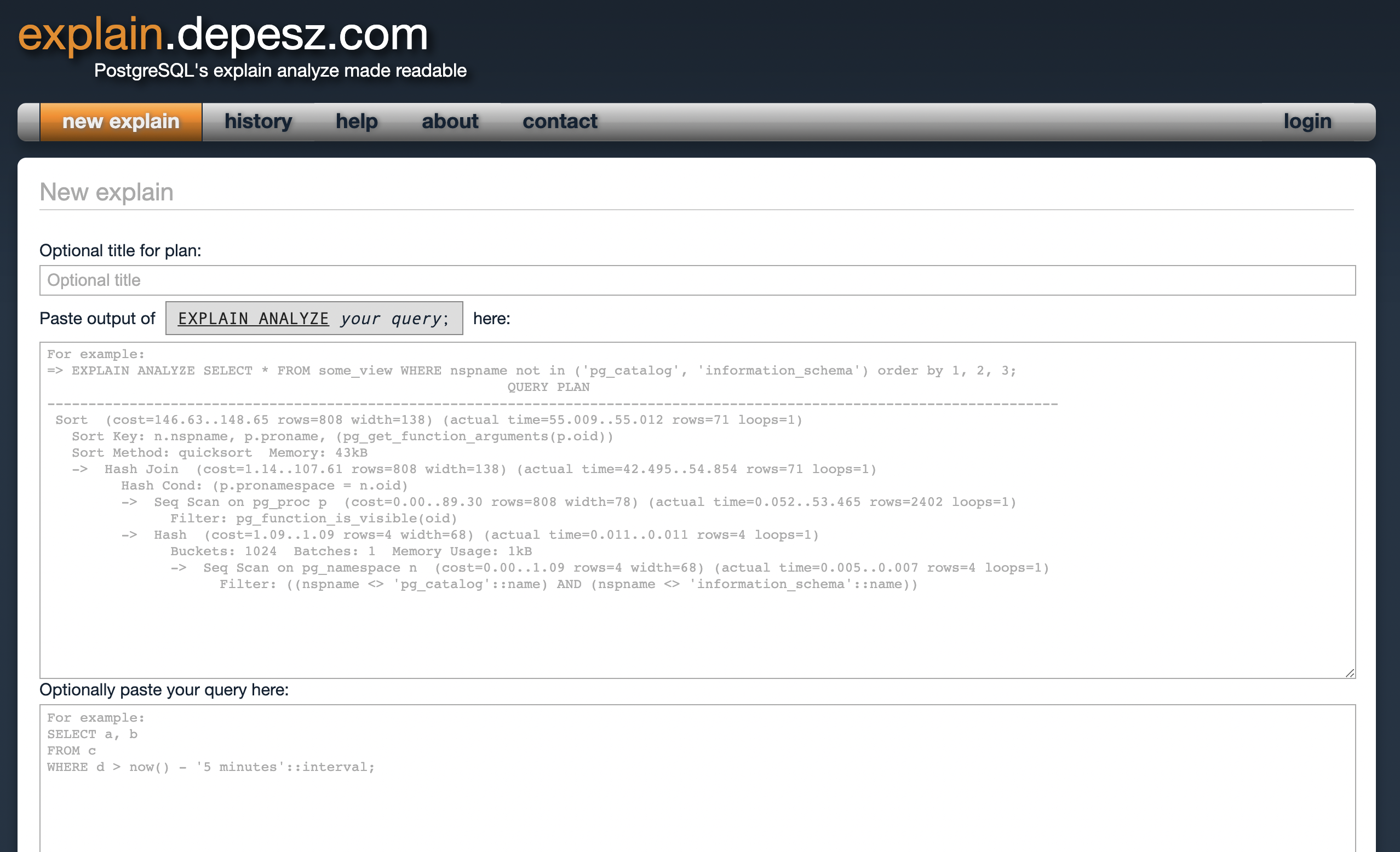
For example, probably the most popular (and definitely the oldest) plan visualization tool, explain.depesz.com, unfortunately, offers to "Paste output of EXPLAIN ANALYZE your query;", ignoring BUFFERS:
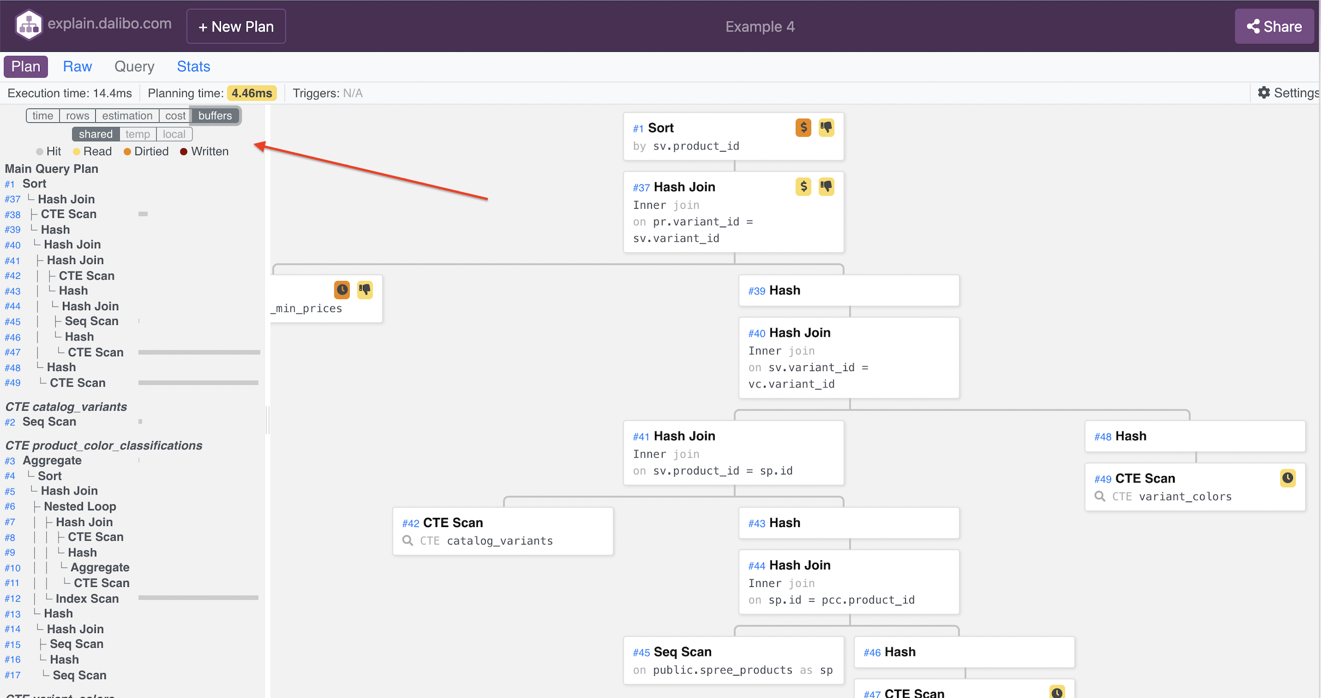
Another visualization tool, explain.dalibo.com, offers: "For best results, use EXPLAIN (ANALYZE, COSTS, VERBOSE, BUFFERS, FORMAT JSON)" and has an interesting additional view on the left side that has the "buffers" option (unfortunately, this view is not default, so a click is required):
Some time ago, I had a conversation with a developer of one of the most popular tools to work with Postgres databases, DBeaver – at that moment, they have just implemented the plan visualization feature. We chatted a bit (#RuPostgres Tuesday, video, in Russian), and he was very surprised to hear that the BUFFERS option matters to me so much.
I recommend all tool developers extend their tools and include BUFFERS by default when working with query plans. In some cases, it makes sense to focus on the BUFFERS metrics.
Ideas for PostgreSQL development
It is a shame that BUFFERS is still not enabled by default in EXPLAIN ANALYZE. I know many people – including experienced DBAs and Postgres maintainers – who support this idea. There are patches proposed to change it. If you are participating in the pgsql-hackers mailing list, consider supporting the idea in this thread and – if you can – reviewing the patch.

DBLab Engine
Instant database branching with O(1) economics.